Inspecting results
Visualizing and inspecting the results of evolutionary strategies (ES) are crucial practices in computational intelligence. Visualization helps in understanding how solutions evolve over generations. Through visual inspection, one can observe if the population is converging towards a global optimum or if it is stuck in local optima. Visualization of the population distribution over time can also highlight issues with diversity, indicating whether the evolutionary strategy is exploring the solution space adequately. pyHMS provides different methods for DemeTree object that enable inspecting results. Let’s consider Sphere function as an example for N=5.
import numpy as np
from pyhms import (
    EALevelConfig,
    hms,
    get_NBC_sprout,
    DontStop,
    MetaepochLimit,
    SEA,
    FunctionProblem,
)

N = 5
square_bounds = np.array([(-20, 20)] * N)
square_problem = FunctionProblem(lambda x: sum(x**2), maximize=False, bounds=square_bounds)

config = [
    EALevelConfig(
        ea_class=SEA,
        generations=2,
        problem=square_problem,
        pop_size=20,
        mutation_std=1.0,
        lsc=DontStop(),
    ),
    EALevelConfig(
        ea_class=SEA,
        generations=4,
        problem=square_problem,
        pop_size=10,
        mutation_std=0.25,
        sample_std_dev=1.0,
        lsc=DontStop(),
    ),
]
global_stop_condition = MetaepochLimit(limit=10)
sprout_condition = get_NBC_sprout(level_limit=4)
hms_tree = hms(config, global_stop_condition, sprout_condition)
The easiest way to inspect the result is to use summary function.
print(hms_tree.summary())
Hello, Sphinx!
Metaepoch count: 10
Best fitness: 4.0969e+01
Best individual: [-0.98073221  5.60137768  1.90436279  0.36727929  2.20676164]
Number of evaluations: 1100
Number of demes: 4

Level 1.
Best fitness: 4.4035e+01
Best individual: [-2.18605631  5.04397642 -0.13939482 -3.07911958  2.07694541]
Number of evaluations: 400
Number of demes: 1

Level 2.
Best fitness: 4.0969e+01
Best individual: [-0.98073221  5.60137768  1.90436279  0.36727929  2.20676164]
Number of evaluations: 700
Number of demes: 3

EADeme root f(-2.19, 5.04, -0.14, -3.08, 2.08) ~= 4.40e+01 evals: 400
├-- EADeme 0 f(-0.95, 7.80, -0.46, -5.37, 2.35) ~= 9.64e+01 sprout: (-3.16, 9.23, -1.03, -6.96, 3.86); evals: 340
├-- EADeme 1 f(-7.85, 5.28, -3.02, 6.66, -4.04) ~= 1.59e+02 sprout: (-9.32, 7.59, -4.32, 7.31, -4.60); evals: 300
└-- EADeme 2 *** f(-0.98, 5.60, 1.90, 0.37, 2.21) ~= 4.10e+01 sprout: (-2.18, 6.20, 2.09, -0.30, 2.38); evals: 60
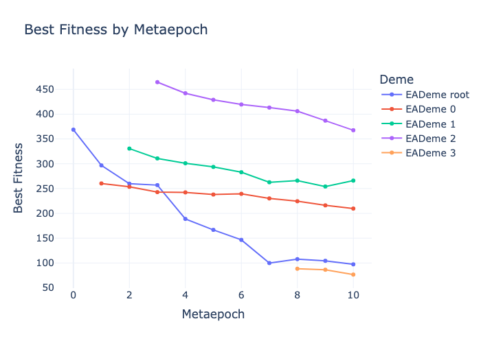
To easily investigate the performance of each deme in the tree, we can use the plot_best_fitness method.
hms_tree.plot_best_fitness()
Analyzing the relationship between distance to the best solution and fitness values can provide valuable insights into the fitness landscape and convergence behavior. For this purpose, you can use the plot_fitness_value_by_distance method.
hms_tree.plot_fitness_value_by_distance(filepath="fitness_by_distance_plot.png", group_by="deme")

This plot shows how fitness changes as the distance from the best solution increases, which helps in understanding the smoothness of the fitness landscape and how well different demes are exploring promising regions. The grouping can be done by either “deme” or “level”.
To visualize the population of individuals across different demes, the plot_population method is useful, especially for 2D problems:
hms_tree.plot_population(filepath="population_plot.png")

This visualization shows the distribution of individuals in the search space. For 2D problems, it plots individuals directly in their coordinate space. Additional options include showing a grid representation of the problem surface, optimal points, and scaling.
Another important aspect of evolutionary strategies is understanding how diversity changes over time. The plot_deme_metric method helps visualize the convergence behavior of a specific deme:
hms_tree.plot_deme_metric(filepath="deme_metric_plot.png")
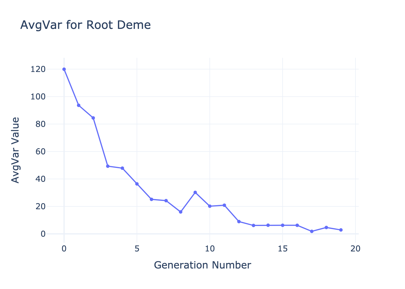
This plot shows how the selected diversity metric changes across generations for a specific deme (root by default). Available metrics include “AvgVar”, “SD”, “SDNN”, and “SPD”. This helps in analyzing exploration versus exploitation behavior.
We can also generate an animation presenting populations of all demes.
hms_tree.animate("your_path.gif")
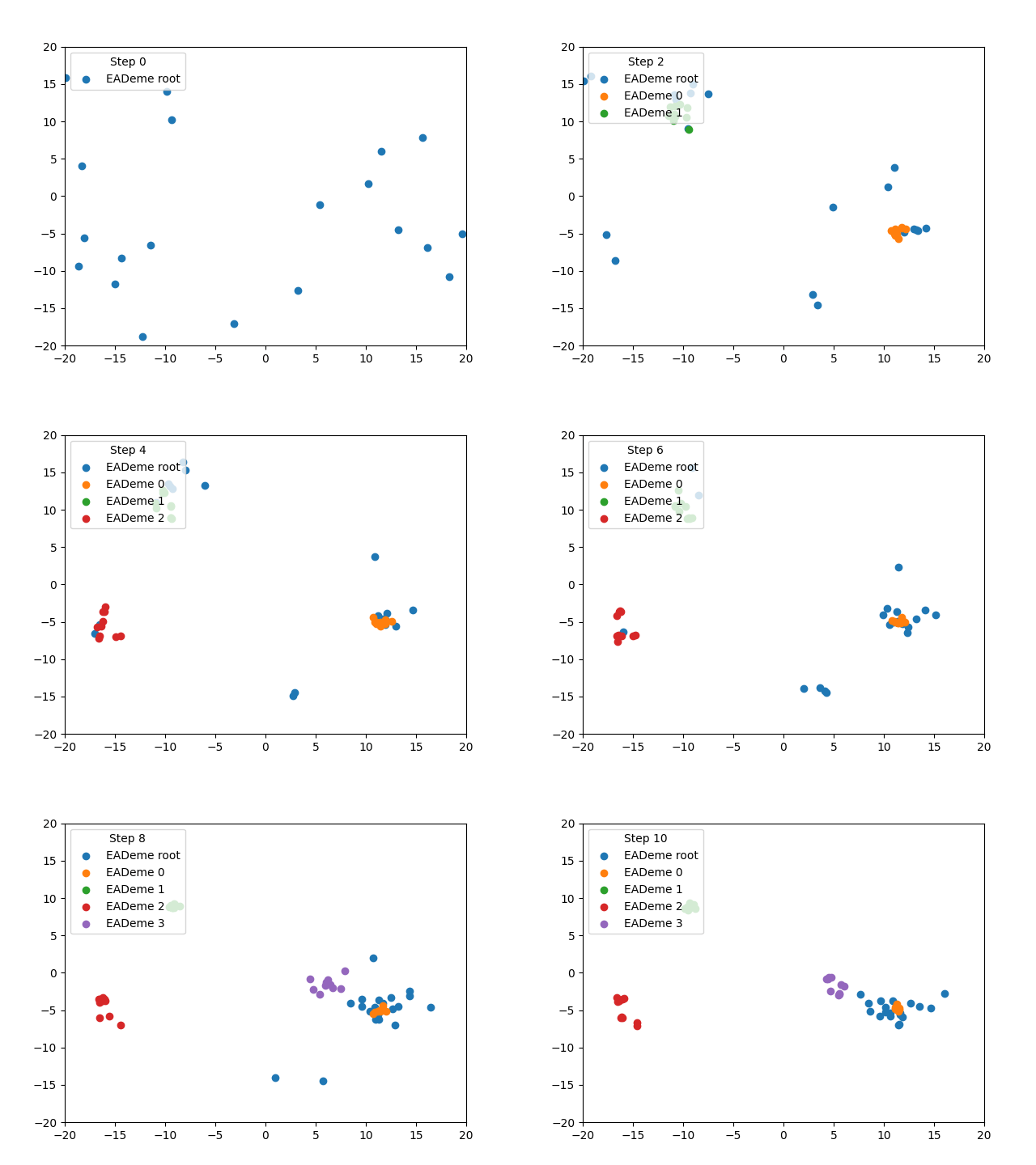
By default for each individual in the population, the first two dimensions are used to visualize the population. To change this behaviour, please specify the dimensionality_reducer parameter.
from sklearn.decomposition import PCA
hms_tree.animate(filepath="your_path.gif", dimensionality_reducer=PCA(n_components=2))
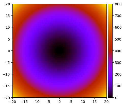
In case of 2D problems, we can visualize the problem itself by plot_problem_surface.
hms_tree.plot_problem_surface()